Optimizing Your Keyboard Layout

I’ve recently gotten into the fabulous world of mechanical keyboards. Other than the Ａｅｓｔｈｅｔｉｃｓ and the fact that building working electronics is cool, the main draw for me was the ability to completely customize how your board works. Just imagine all the chances for increased ｐｒｏｄｕｃｔｉｖｉｔｙ!

Of course, good cognitive scientist as I am, I know that optimal performance requires a good grip of the statistics of the environment you’re working in. For us, that’s going to be our typing patterns! Here, I’ll show you how I was able to capture a huge amount of data on how I type, how to play around with it, and how to do the same for your own keyboard.

My set up

This tutorial/demonstration is for those who know something about mechanical keyboards, and just a little bit about the QMK firmware that powers most custom boards. I’m relatively new to QMK myself, but I’m trying to make things a little bit easier for the next guy. However, I’m not a developer for this project, and my free time is limited, so this will be specific to my experience and setup, etc.

After suffering through the hell that was the Massdrop group buy for Jack Humbert’s Planck mechanical keyboard¹, I’ve finally got a fully programmable keyboard of my own. This guide will be for that rev4 Planck. I use an old Macbook Pro with OSX 10.9.5 (I really need to get around to updating!) and R version 3.3.1 (more shame!).

I can tell you right now, following this tutorial on a PC is going to be challenging. Making and flashing custom QMK layouts to your keyboard is way easier on Unix-based systems, and most of the cool open-source stuff is for Unix as well. Now is the perfect time to get in on that Linux action if you haven’t already. Installing a virtual machine on your PC is a commitment-free way of playing around with Linux, and I’d recommend that.

Getting your typing data

Alright folks, this here’s the secret I learned: download selfspy. Selfspy is basically spyware you use on yourself–it collects enormous amounts of information on your activity on your computer. It records every keystroke, every name of every window you open, and your mouse movements as well. Unlike spyware, it doesn’t send this data to anybody else, it just saves all of it in an Sqlite database on your computer.

Installing selfspy

Heads up: this might not that be easy to do. I kinda blacked out from the stress of trying to get it installed right, so my memory about what I did to get it to work is a little hazy. Follow the instructions on the Github page as well as you can, but IIRC I had to install the exact versions of some of the stuff listed in the osx_requirements.txt file. In particular, I think I had to make sure I was using the 3.0.4 version of pyobjc in the end (I used the pip installer).

Looking back, you might be able to just update the pyobjc requirements in osx_requirements.txt to whatever you have currently, but I’m not positive about that.

Analyzing your data

Open up a terminal, and run selfspy to have it start collecting your data. A word to the wise: unless you sometimes pause it, it will record EVERYTHING. All your passwords, the names of all those dirty, dirty sites you visit (you filthy animal!)–everything.

This isn’t a such a big deal, however, because you can have it encrypt the data it stores in the database on your computer. If you’re fine with somewhat surface-level analyses of your data, this is fine–selfspy comes with a program called selfstats that lets you print out some basic analyses of your data, including key frequencies. If you want to see how often you’ve pressed each key while selfspy has been running, you can do it with selfstats easy-peasy.

But if you want to manipulate all that juicy, succulent data yourself (you little pervert!), the fact that it’s all encrypted is a bit of problem. At least it was for me, who doesn’t know how to decrypt it with the tools I had on hand. Instead, I opted to just leave everything unencrypted and pray to God that the Russians don’t get a hold of my computer². The R code that I’ve written to analyze the data at a more fine-grain level only works when it’s unecrypted, so either figure out how to decrypt Blowfish in R or Python, or let your freak flag fly.

Walking through my code

I do a lot of R coding and use Hadley Wickham’s beautiful R babies all the time. One of his packages, dplyr, has³ the capability of manipulating SQL data, so that’s what I use to access the data stored in ~/.selfspy/selfspy.sqlite. I’ll run you through some of it so you can get a sense of how it works. You can download it for yourself in the link at the end of the post–it comes with (hopefully) helpful comments and multiple examples for you to acquaint yourself with different possibilities.

library(dplyr) # you should add `library(dbplyr)` if you're using the newest version of dplyr
library(tidyr)
library(stringr)
library(purrr)

# Loading in the data from a personalized (smaller) database
selfspy_db <- src_sqlite("~/.selfspy/selfspy_post.sqlite", create = T)
# Below is the default location for the database, and what you would presumably use
# selfspy_db <- src_sqlite("~/.selfspy/selfspy.sqlite", create = T)
selfspy_db

## src:  sqlite 3.11.1 [~/.selfspy/selfspy_post.sqlite]
## tbls: click, geometry, keys, process, window

You can see that there are five tables in the database: click (mouse data?), geometry (window size data?), keys (key press data), process (the names of the programs), window (data on what windows have been active). For this excursion, we’ll only care about keys and process.

Note: For this demonstration, I’m using a smaller copy of one of my databases. This is because: 1) I accidentally locked myself out of my month-long database and 2) I don’t want any weird stuff being coming up in this tutorial!

# Opening connections to the key and process databases
key_db <- tbl(selfspy_db, "keys")
process_db <- tbl(selfspy_db, "process")

key_db

## Source:   query [?? x 10]
## Database: sqlite 3.11.1 [~/.selfspy/selfspy_post.sqlite]
## 
##       id                 created_at        text
##    <int>                      <chr>      <list>
## 1      1 2017-10-18 14:24:13.692624  <raw [12]>
## 2      2 2017-10-18 14:24:28.915149  <raw [24]>
## 3      3 2017-10-18 14:24:30.259072  <raw [12]>
## 4      4 2017-10-18 14:25:05.551297  <raw [42]>
## 5      5 2017-10-18 14:27:39.875412 <raw [397]>
## 6      6 2017-10-18 14:27:50.265004  <raw [27]>
## 7      7 2017-10-18 14:27:57.575051  <raw [48]>
## 8      8 2017-10-18 14:27:59.317140  <raw [12]>
## 9      9 2017-10-18 14:28:00.678074  <raw [13]>
## 10    10 2017-10-18 14:28:02.835207  <raw [19]>
## # ... with more rows, and 7 more variables: started <chr>,
## #   process_id <int>, window_id <int>, geometry_id <int>,
## #   nrkeys <int>, keys <list>, timings <list>

See the Source: query [?? x 10] at the top? As it currently stands, key_db isn’t a data frame or a tbl_df–it’s just a query to the database–it doesn’t know how many rows there are yet. When dealing with SQL, dplyr evaluates things lazily, meaning it won’t actually fetch all the data from the database unless you demand it.

You can see that there’s a lot of info in key_db: in addition to timing information for the key presses, it has the IDs of all the applications and windows that were active while you were typing. Today, I’ll only be focusing on the key presses and the names of the applications.

Let’s look at some of the functions I’ve written to help you analyze your data.

Getting the key presses in human-readable formats

In order analyze the key presses, we have to get them to a point where we can work with them. For this, I’ve written the function getPresses(). There are a lot of optional arguments, but they’re detailed in the code. The basic functionality is like this:

getPresses(key_db) %>%
  select(cleanStrings) # selecting only the "cleaned up" version of the key presses

## # A tibble: 110,389 × 1
##    cleanStrings
##           <chr>
## 1  <[Cmd: Tab]>
## 2             a
## 3             a
## 4             a
## 5             a
## 6             s
## 7             s
## 8             s
## 9             s
## 10            a
## # ... with 110,379 more rows

For those of you not used to R and those R users not used to the tidyverse, the %>% operator pipes the output of everything on the left of it (getPresses(key_db)) into the function on the right of it as the first argument (or, wherever you put a .). Thus, what is above is equivalent to select(getPresses(key_db), cleanStrings). My irrational commitment to never declare new variables might make some of the code seem a little weird to some of you–each function is basically a single “flow”.

Understanding the output: basic

The output from getPresses() is essentially a table where every row is a single key press (kind of). The keypresses are saved as strings with the “cleaned up” version of each press in the cleanStrings column. A row with “a” in this column means you typed that character–unfortunately, selfspy includes the presence of the Shift key in this value, so “A” actually means Shift + 'a'. For modifier combos and certain other key presses, such as Command + Tab or Backspace, the key press is saved in brackets like <[Cmd: Tab]>. Technically speaking, these probably aren’t “key presses”–selfspy doesn’t record pressing the Command, Alt, or Ctrl keys unless they are pressed along with some other key.

By itself, the output of getPresses is pretty useless. If we want to analyze the data, maybe we’d want to start looking at which keys are pressed the most often, or what shortcuts are used the most. That way, we could decide how accessible each key should be on our keyboard, or what shortcut macros might help the most.

To get a sense of this, I’ve created a function called getStats():

key_db %>% 
  getPresses() %>%
  getStats(s_col="cleanStrings", # The name of the column of the key press strings being passed in
           break_multitaps=TRUE # This will ungroup repeated taps (see below)
           ) %>%
  arrange(-n) # order the keys with the highest frequencies on top

## Source: local data frame [201 x 3]
## Groups: cleanStrings [201]
## 
##     cleanStrings areModsPressed     n
##            <chr>          <dbl> <dbl>
## 1       <[Down]>              1 27490
## 2  <[Backspace]>              1 13940
## 3                             0 13431
## 4              e              0  7953
## 5              t              0  6296
## 6              a              0  5281
## 7              o              0  4844
## 8              i              0  4626
## 9              s              0  4584
## 10             n              0  4332
## # ... with 191 more rows

You can see from the output that there are three columns: the names of the key presses, areModsPressed (a column indicating whether functional/modifier keys were pressed down, excluding Shift), and n (the number of presses).

It seems that so far, I press “Down” and “Backspace” the most, followed by “Space” (annoyingly represented as actual whitespace) and then some really common letters. (You can show all the rows by piping the output into as.data.frame().) Not super surprising. But we set the break_multitaps to TRUE–what was up with that?

Well, selfspy automatically records repeated “bracketed” key presses with a single entry. So 15 Command + Tabs in a row will be recorded as <[Command + Tab]x15>. By default, getStats() treats this as a single key press. This is useful if you want to consider making macros for, say, something that presses Backspace three times in a row. Note that only “bracketed” key presses are recorded this way. By setting break_multitaps=TRUE, we treat these repeated presses individually.

Understanding the output: intermediate

But what if you’re not satisfied with something that you could basically do with the selfstats command? For example, what if you wanted to look at how you typed differently in different applications (perhaps for creating a Python layer or an R layer), or if you wanted to look at multi-press patterns?

I’ve made getPresses() capable of separating key presses by application name, so that they can be analyzed independently in parallel. Here we use our old friend process_db from earlier. Because the key_db only has numbers for each process, if we want to see the names those numbers refer to, we have to pass in what is essentially a number-to-name dictionary (process_db, after we call collect() on it).

key_db %>% 
  getPresses(process_id_df    = process_db %>% # so we can use application names rather than numbers for process IDs
               select(-created_at) %>% # I remove a column that we don't need
               collect(), # this function makes dplyr stop being lazy and fetch us the actual data
             group_by_process = TRUE)

## # A tibble: 22 × 2
##             process_id                  data
##                  <chr>                <list>
## 1             Terminal  <tibble [5,103 × 8]>
## 2              RStudio <tibble [34,689 × 8]>
## 3        Google Chrome <tibble [39,471 × 8]>
## 4         TextWrangler  <tibble [3,097 × 8]>
## 5               Finder    <tibble [580 × 8]>
## 6             TextEdit  <tibble [5,213 × 8]>
## 7                Notes  <tibble [1,851 × 8]>
## 8          QMK Flasher      <tibble [3 × 8]>
## 9  CoreServicesUIAgent      <tibble [1 × 8]>
## 10     Microsoft Excel    <tibble [151 × 8]>
## # ... with 12 more rows

A marvel of the tidyverse is that it can store entire data frames as single cells in bigger data frames. Each cell in the data column above is a data frame of all the key presses for the application in the process_id column.

We can analyze each of these data frames the same as we would a single data frame with Hadley Wickham’s purrr package. Having started my programming journey in Scheme, I love me some functional programming. The map function in purrr lets us apply the getStats function to the inside of each data frame in the data column.

key_db %>% 
  getPresses(process_id_df = process_db %>% select(-created_at) %>% collect(), 
             group_by_process = TRUE) %>%
  mutate(data = purrr::map(data, ~getStats(., # Don't forget the tilde in front of the function, and you have to use the '.' to indicate where the first argument of `purrr::map` should appear
                                           s_col="cleanStrings",
                                           break_multitaps=FALSE))) %>%
  tidyr::unnest() %>% # Expands the data frames in the `data` column
                      # If you want to keep them separate, keep manipulating them with `map`!
  arrange(-n)

## # A tibble: 2,230 × 4
##        process_id cleanStrings     n areModsPressed
##             <chr>        <chr> <int>          <dbl>
## 1   Google Chrome               4952              0
## 2         RStudio               4129              0
## 3   Google Chrome            e  3014              0
## 4         RStudio            e  2493              0
## 5   Google Chrome            t  2360              0
## 6  Microsoft Word               2151              0
## 7   Google Chrome            o  2023              0
## 8         RStudio            t  1971              0
## 9   Google Chrome            a  1949              0
## 10  Google Chrome            i  1797              0
## # ... with 2,220 more rows

Yeah, most of my typing is typing English words, separated by spaces, so you can see similar statistics for the top key presses across applications.

There are differences, however. I threw together this quick-and-dirty little visualization that compares the highest key presses across applications.

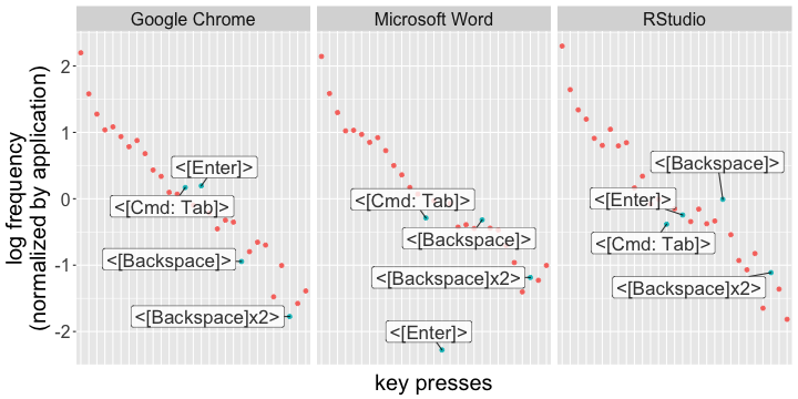
Visualizing the most-pressed keys across a few applications. Presses with modifier keys are highlighted--the rest are boring and left blank. The order of the keys is identical across applications. Note the dearth of returns in Word--it's probably because I'm writing in paragraphs as opposed to coding/browsing.

It’s a pretty boring plot for the most part (sue me!), but you can see some differences emerging across applications. I press the Enter key a lot less in Microsoft Word, than I do when I’m coding in R, or browsing the web. Presumably, that’s because I type in paragraphs in Word. If I want to optimize my key layout, I might be ok with making a layer for Word where the Enter key is less accessible.

I urge you to really play around with your data at this point. Really get in there and see what’s up. You can do a lot of comparisons between applications, visualize it, etc.–I’ve really only shown the most boring possibilities above. The differences get much more interesting once you get past the alpha keys.

Understanding the output: advanced

What would a rational keyboard layout look like? I’m tempted to start prattling on about what that could be, bringing in concepts from information theory or psycholinguistics, but to spare you my philosophizing, I’ll just settle on a super basic definition: a rational keyboard layout is one that minimizes the number of necessary key strokes for the statistics of the output and the constraints of the board⁴.

Ugh, it’s too hard to stop myself from going into lecture mode, so I’ll just say this–if you type the same multi-key patterns again and again, why not reduce them to fewer key presses? For example, I type the %>% operator a lot in R–maybe I want to make this a macro that I can press with a single button? Well, if you want to start looking at key press n-grams, I wrote some rudimentary code for that as well!

The function nGramPresses() basically does the same thing as getPresses(), but it clusters subsequent key-presses into groups of n. Let’s look at what happens when we analyze the frequency of 4-gram key presses that use modifier keys, grouping them by application.

key_db %>% 
  nGramPresses(process_id_df    = process_db %>% select(-created_at) %>% collect(), 
               group_by_process = TRUE,
               n=4) %>% # n is an integer greater than 0
  mutate(data = purrr::map(data, ~getStats(., 
                                           s_col="cleanStrings", 
                                           break_multitaps=FALSE))) %>% # `break_multitaps` needs to be set to false if you're using n-grams. If you have the know-how, you could pretty easily change the code so that it works
  tidyr::unnest() %>% 
  arrange(-n) %>% 
  filter(areModsPressed!=0) %>% 
  head(10) %>% as.data.frame()

##       process_id            cleanStrings  n areModsPressed
## 1       Terminal         <[Enter]>-g-i-t 67              1
## 2        RStudio         %->-%-<[Enter]> 55              1
## 3       Terminal         <[Enter]>-c-d-  54              1
## 4       Terminal <[Enter]>-l-s-<[Enter]> 48              1
## 5       Terminal         l-s-<[Enter]>-c 46              1
## 6       Terminal         s-<[Enter]>-c-d 40              1
## 7        RStudio    <[Cmd: Enter]>- -%-> 27              1
## 8       Terminal         t-u-s-<[Enter]> 25              1
## 9       Terminal   <[Tab]>-<[Enter]>-l-s 24              1
## 10 Google Chrome         r-e-d-<[Enter]> 24              1

Look at that! Now we’re getting somewhere! You can get a sense of what I’ve been doing the most from these n-grams! I’ve been using git a lot (e.g., <[Enter]>-g-i-t), navigating with the terminal (with ls and cd), and yes, it looks like I do use the %>% operator (followed by a return) a lot! Hilariously, you can also see my reddit obsession: I just type r-e-d to get the autocomplete suggestions, and then press Enter!

Other layouts

Hopefully, I’ll be getting around to writing a newbie’s introduction to QMK, but for those of you with no C++ experience, check out kbfirmware.com for an easy way to make basic layers and layouts. For those who are just starting out on their QMK journey, my advice is to copy the hell out of other people’s code and layouts–there are loads of examples for most keyboards in the firmware!

There are also great ideas to draw inspiration from. For example, my current layout (which you can follow along with here) draws a lot of inspiration from Noah Frederick’s set up. This person also has a bunch of crazy layouts and code that beginners might find helpful.

If this helps at all, or if you have any questions (please don’t be about installing selfspy please don’t be about installing selfspy), feel free to drop a comment here or on reddit!

Source Code:

keyboard_analysis.R

The code that I banged out for this project. Although it’s using some outdated package versions, I added a lot of comments and usage examples.

2017-10-28-selfspy_post.Rmd

The R Markdown file this blog post is generated from, if you want to know what R code I used for the plot, etc.

Footnotes